Computational Mathematics and Analysis
CFD Example Work
2018
This project demonstrates my capabilities in computational mathematics and analysis. I used MATLAB to solve this problem, but I have equally used Python on other project. The following computations and results solve the classical problem of a square cavity with an incompressible flow driven by a lid moving at a constant velocity. The solution obtains nondimensional forms of the vorticity transport equation and the Poisson equation using a characteristic length of L and characteristic velocity of Ulid. These functions are discretized using second-order central difference in space and forward Euler in time. The boundary conditions are established as shown below where ω is vorticity and Ψ is stream function. The code begins with all zero initial conditions except at the moving boundary, then iterates in time until the flow reaches steady state to within a tolerance of 10E-6 in the L2-norm.
Setup

Results

Measure of local rotation

Constant magnitudes are streamlines
(Unitless)
Measure of local rotation
Code
%Taber Miyauchi
%Computational Fluid Dynamics
%4-25-18
%Incompressible, 2D, Constant Property Flow:
%Classical Lid-Driven Square Cavity Problem Using Vorticity Stream Function
clc;
close all;
clear all;
format compact;
%%Given
Re = 300; % Reynold's number
U = 1; % Velocity of lid
dt = .006; % Time step
h = .05; % Spacing of element nodes (Grid size)
x = 0:h:1; % Horizontal length
y = 0:h:1; % Vertical length
%Code Setup
t_norm = Inf; % Initializing change in velocity between time steps
tol = 10e-6; % Tolerance of t_norm
iteration = 0; % Iteration counter
%Initial Conditions
u = zeros(length(y),length(x)); % Horizontal velocity
u(length(y),:)=1; % Velocity driven by lid
v = zeros(length(y),length(x)); % Vertical velocity
u_new = u; % New horizontal velocity after one compute iteration
v_new = v; % New vertical velocity after one compute iteration
Ps = zeros(length(y),length(x)); % Stream function (psi)
w = zeros(length(y),length(x)); % Vorticity (omega)
w_new = zeros(length(y),length(x)); % Vorticity after one computational iteration
%Boundary Conditions
%Left Side
u(:,1) = 0;
v(:,1) = 0;
Ps(:,1) = 0;
%Bottom Side
u(1,:) = 0;
v(1,:) = 0;
Ps(1,:) = 0;
%Right Side
u(:,length(x)) = 0;
v(:,length(x)) = 0;
Ps(:,length(x)) = 0;
%Top Side
v(length(y),:) = 0;
Ps(length(y),:) = 0;
%% Computation
while t_norm > tol
%% Calculating vorticity
%Discretized (First-order, One-Sided Difference) vorticity boundary conditions
w(:,1) = 2*(-Ps(:,2)+Ps(:,1))/(h^2); %Left Side
w(1,:) = 2*(-Ps(2,:)+Ps(1,:))/(h^2); %Bottom Side
w(:,length(x)) = 2*(Ps(:,length(x))-Ps(:,length(x)-1))/(h^2); %Right Side
w(length(y),:) = 2*(Ps(length(y),:)-Ps(length(y)-1,:)-U*h)/(h^2); %Top Side
%Updating vorticity boundary conditions
w_new(:,1) = w(:,1); %Left Side
w_new(1,:) = w(1,:); %Bottom Side
w_new(:,length(x)) = w(:,length(x)); %Right Side
w_new(length(y),:) = w(length(y),:); %Top Side
%Calculating inner components of vorticity
for i = 2:length(x)-1;
for j = 2:length(y)-1;
%Discretized (2nd-Order Central in space, FE in time) vorticity transport equation
w_new(j,i) = w(j,i) + dt*((-u(j,i)*(w(j,i+1)-w(j,i-1))/(2*h))-...
(v(j,i)*(w(j+1,i)-w(j-1,i))/(2*h))+ 1/Re*(((w(j,i+1)-2*w(j,i)+...
w(j,i-1))/h^2)+((w(j+1,i)-2*w(j,i)+w(j-1,i))/h^2)));
end
end
w = w_new;
%% Calculating stream function
%Using Gauss-Seidel Method
%Calculating left to right, bottom to top
normValue = Inf; %Initialize change is stream function
while normValue > tol
Ps_old = Ps;
for i = 2:(length(x)-1);
for j = 2:(length(y)-1);
%Discretized (2nd-Order Central diff in space) Poisson equation
Ps(j,i) = 1/4*(Ps_old(j+1,i)+Ps(j-1,i)+...
Ps_old(j,i+1)+Ps(j,i-1)+w_new(j,i)*h^2);
end
end
normValue = norm(Ps_old-Ps);
end
%% Calculating velocity
for i = 2:length(x)-1;
for j = 2:length(y)-1;
%Discretized (2nd-Order Central diff in space) stream function equation
v_new(j,i) = -(Ps(j,i+1)-Ps(j,i-1))/(2*h);
u_new(j,i) = (Ps(j+1,i)-Ps(j-1,i))/(2*h);
end
end
%Checks for steady state
t_norm = norm(u-u_new);
iteration = iteration + 1;
%Updating velocity
v = v_new;
u = u_new;
end
%% Plot
figure(1);
contourf(x,y,Ps,20);
axis('equal');
xlabel('X Location');
ylabel('Y Location');
colormap(jet)
colorbar
ylabel(colorbar,'Stream Function Contours','FontSize', 10);
title('\bf Stream Function of Cavity');
figure(2);
contourf(x,y,w_new,25)
axis('equal');
xlabel('X Location');
ylabel('Y Location');
colormap(jet)
colorbar
ylabel(colorbar,'Vorticity Contours','FontSize', 10);
title('\bf Vorticity of Cavity');
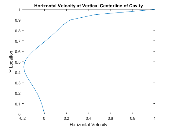
u_center = u_new(:,(length(x)+1)/2);
figure(3);
plot(u_center,y);
xlabel('Horizontal Velocity');
ylabel('Y Location');
title('\bf Horizontal Velocity at Vertical Centerline of Cavity');